|
You are here : Control System Design - Index | Simulations | Tank Level | Part 1 Tank Level Tutorial - Part 1Before continuing, make sure you have read Chapter 7 and Chapter 19. System ModelBefore we continue with the observer design, we must make a model of the system. The height of tank 1 can be described by the equation
Similarly, h2 is given by
The flow between the two tanks can be approximated by the free fall velocity for the difference in height between the two tanks.
Now, if we measure the heights of the tanks in % (where 0% is empty and 100% is full), we can convert the flow rates into equivalent values in % per second (where f1 is the equivalent flow into tank 1 and f2 is the equivalent flow out of tank 2). The model for the system is
where
We can then choose to linearise this model for a nominal steady state height difference (or operating point). Let
then
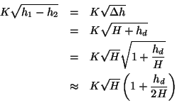
since
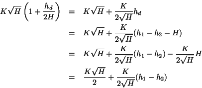
then
This yields the following linear model
where
Since we are assuming that h2 can be measured and h1 cannot, we set C = [ 0 1 ] and D = [ 0 0 ]. The resulting system is both controllable and observable (which you can easily verify). Now we wish to design an observer
to estimate the value of h2. The characteristic polynomial of the observer is
so we can choose the observer poles which gives us values for J1 and J2. If we assume that the operating point is H = 10%, then k = 0.0411. If we wanted poles at s = -0.9822 and s = -0.0531, then we would calculate that J1 = 0.3 and J2 = 0.9. If we wanted two poles at s = -2, then J1 = 3.9178 and J2 = 93.41. The equation for the observed system is then
Where where Alternatively, we could use the non-linear model in our observer to attempt to get better performance:
Java Applet SimulationThe JAVA applet below is a simulation of the above tank system. The purpose of this simulation is to investigate the difference between the linear and non-linear observers. Thus, we will not concern ourselves with the controller at this stage. The graph has a vertical scale of 25% per division and a horizontal scale of 10 sec per division. It shows the set-point (the orange trace), the actual h1 (the blue trace), the estimated h1 (the red trace) and the actual h2 (the green trace). Pressing the "Change Parameters" button allows you to change the set point type, the measurement noise level, the type of observer (linear or non-linear) and the observer gain matrix J.
By pushing the observer poles out towards negative infinity, we get a faster response from the observer, but we also change the sensitivity to modelling errors (particularly relevant in the linear observer) and measurement noise. By now, this should be a familiar trade-off. |
||||||||


