|
You are here : Control System Design - Index | Book Contents | Appendix D | Section D.1 D. Properties of Continuous-Time Riccati Equations
|
![\begin{displaymath}
\ensuremath{\mathbf{P}} (t)=\ensuremath{\mathbf{N}} (t)[\ensuremath{\mathbf{M}} (t)]^{-1}
\end{displaymath}](appendixD-img8.png)
 and
and
 satisfy the following equation:

![\begin{displaymath}
\ensuremath{\mathbf{N}} (t_f)[\ensuremath{\mathbf{M}} (t_f)]^{-1}=\ensuremath{\boldsymbol{\Psi}} _f
\end{displaymath}](appendixD-img12.png)
![\begin{displaymath}
\frac{d\ensuremath{\mathbf{P}} (t)}{dt}=\frac{d\ensuremath{...
...\mathbf{N}} (t)\frac{d[\ensuremath{\mathbf{M}} (t)]^{-1}}{dt}
\end{displaymath}](appendixD-img13.png)
![$[\ensuremath{\mathbf{M}} (t)]^{-1}$](appendixD-img14.png) can be computed by noting
that
can be computed by noting
that
![$\ensuremath{\mathbf{M}} (t)[\ensuremath{\mathbf{M}} (t)]^{-1}=\ensuremath{\mathbf{I}} $](appendixD-img15.png) ;
then
;
then
![\begin{displaymath}\frac{d\ensuremath{\mathbf{I}} }{dt}=\ensuremath{\mathbf{0}} ...
...\mathbf{M}} (t) \frac{d[\ensuremath{\mathbf{M}} (t)]^{-1}}{dt}
\end{displaymath}](appendixD-img16.png) |
(D.1.5) |
from which we obtain
![\begin{displaymath}\frac{d[\ensuremath{\mathbf{M}} (t)]^{-1}}{dt}=-[\ensuremath{...
...uremath{\mathbf{M}} (t)}{dt}[\ensuremath{\mathbf{M}} (t)]^{-1}
\end{displaymath}](appendixD-img17.png) |
(D.1.6) |
Thus, Equation (D.1.4) can be used with (D.1.2) to yield
![\begin{displaymath}
\begin{split}
- \frac{d\ensuremath{\mathbf{P}} (t)}{dt}&=\e...
...h{\mathbf{N}} (t)[\ensuremath{\mathbf{M}} (t)]^{-1}
\end{split}\end{displaymath}](appendixD-img18.png)
which shows that
 also satisfies
(D.0.1), upon using (D.1.1).
also satisfies
(D.0.1), upon using (D.1.1).
The matrix on the right-hand side of (D.1.2), namely,
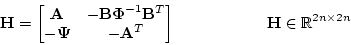
is called the Hamiltonian matrix associated with this problem.
Next, note that (D.0.1) can be expressed in compact form as
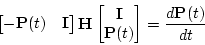
Then, not surprisingly, solutions to the CTDRE, (D.0.1), are intimately connected to the properties of the Hamiltonian matrix.
We first note that
 has the following reflexive property:
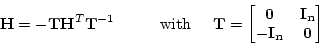
where
 is the identity matrix in
 .
.
Recall that a similarity transformation preserves the eigenvalues;
thus, the eigenvalues of
are the same as those of
 .
On the other hand, the eigenvalues of
and
.
On the other hand, the eigenvalues of
and
 must be the same. Hence, the spectral set of
is
the union of two sets,
must be the same. Hence, the spectral set of
is
the union of two sets,  and
and  ,
such that, if
,
such that, if
 ,
then
,
then
 .
We assume that
does not contain any eigenvalue on the imaginary axis
(note that it suffices, for this to occur, that
.
We assume that
does not contain any eigenvalue on the imaginary axis
(note that it suffices, for this to occur, that
 be stabilizable and that the pair
 have no undetectable poles on
the stability boundary). In this case,
can be so
formed that it contains only the eigenvalues of
that lie
in the open LHP. Then, there always exists a nonsingular
transformation
have no undetectable poles on
the stability boundary). In this case,
can be so
formed that it contains only the eigenvalues of
that lie
in the open LHP. Then, there always exists a nonsingular
transformation
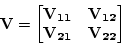
 such that
![\begin{displaymath}[\ensuremath{\mathbf{V}} ]^{-1} \ensuremath{\mathbf{H}}\ensur...
...nsuremath{\mathbf{0}} & \ensuremath{\mathbf{H_u}} \end{bmatrix}\end{displaymath}](appendixD-img34.png)
where
 and
and
 are diagonal matrices with
eigenvalue sets
and ,
respectively.
are diagonal matrices with
eigenvalue sets
and ,
respectively.
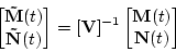
We can use
 to transform the matrices
 and
and
 ,
to obtain
,
to obtain
Thus, (D.1.2) can be expressed in the equivalent form:
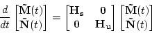
If we partition
in a form consistent with the matrix Equation (D.1.13), we have that
The solution to the CTDRE is then given by the following lemma.
Lemma D.2 A solution for Equation (D.0.1) is given by
![\begin{displaymath}
\ensuremath{\mathbf{P}} (t)= \ensuremath{\mathbf{P_1}} (t) [\ensuremath{\mathbf{P_2}} (t)]^{-1}
\end{displaymath}](appendixD-img43.png)
where

![\begin{displaymath}
\ensuremath{\mathbf{P_2}} (t)=\bigl[\ensuremath{\mathbf{V_{...
...mathbf{V_a}} e^{\ensuremath{\mathbf{H_s}} (t_f-t)}\bigr]^{-1}
\end{displaymath}](appendixD-img45.png)
![\begin{displaymath}
\ensuremath{\mathbf{V_a}}\stackrel{\rm\triangle}{=}-[\ensure...
...(t_f)\left[\ensuremath{\mathbf{\tilde{M}}} (t_f) \right]^{-1}
\end{displaymath}](appendixD-img46.png)
Proof
From (D.1.12), we have
 |
Hence, from (D.1.3),
![\begin{displaymath}\left[
\ensuremath{\mathbf{V}} _{21}\ensuremath{\mathbf{\til...
...lde{N}}} (t_f)\right]
^{-1}
=\ensuremath{\boldsymbol{\Psi}} _f
\end{displaymath}](appendixD-img49.png)
or
![\begin{displaymath}\left[
\ensuremath{\mathbf{V}} _{21}+\ensuremath{\mathbf{V}}...
...}} (t_f)]^{-1}\right]
^{-1}=\ensuremath{\boldsymbol{\Psi}} _f
\end{displaymath}](appendixD-img50.png)
or
![\begin{displaymath}\ensuremath{\mathbf{\tilde{N}}} (t_f)[\ensuremath{\mathbf{\ti...
...\ensuremath{\mathbf{V}} _{11}\right] =\ensuremath{\mathbf{V_a}}\end{displaymath}](appendixD-img51.png)
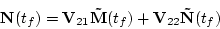
Now, from (D.1.10),
![\begin{displaymath}=\left[ \ensuremath{\mathbf{V}} _{21}\ensuremath{\mathbf{\til...
...12}\ensuremath{\mathbf{\tilde{N}}} (t)\right] ^{-1} \nonumber
\end{displaymath}](appendixD-img52.png) |
![\begin{displaymath}=\left[ \ensuremath{\mathbf{V}} _{21}+\ensuremath{\mathbf{V}}...
...nsuremath{\mathbf{\tilde{M}}} (t)]^{-1}\right] ^{-1} \nonumber
\end{displaymath}](appendixD-img53.png) |
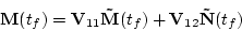
and the solution to (D.1.13) is
 |
Hence,
![\begin{displaymath}\ensuremath{\mathbf{\tilde{N}}} (t)[\ensuremath{\mathbf{\tild...
...f{\tilde{M}}} (t_f)]^{-1}e^{\ensuremath{\mathbf{H}} _s(t_f-t)}
\end{displaymath}](appendixD-img56.png)
Substituting (D.1.25) into (D.1.23) gives the result.
