|
You are here :
Control System Design - Index | Book Contents |
Appendix D
| Section D.2
D. Properties of Continuous-Time Riccati Equations
D.2 Solutions of the CTARE
The Continuous Time
Algebraic Riccati Equation (CTARE) has
many solutions, because it is a matrix quadratic equation. The
solutions can be characterized as follows.
Lemma D.3
Consider the following CTARE:
 |
(D.2.1) |
| (i) |
The CTARE can be expressed as |
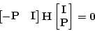 |
(D.2.2) |
|
|
where
 is defined in (D.1.8).
|
| (ii) |
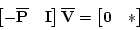
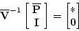
Let
 be defined so that
 |
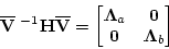 |
(D.2.3) |
|
|
where
 are any partitioning of the
(generalized) eigenvalues of
such that, if
are any partitioning of the
(generalized) eigenvalues of
such that, if  is
equal to
is
equal to
 for same
  ,
then ,
then
 for some
  . .
|
|
Let |
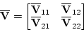 |
(D.2.4) |
|
|
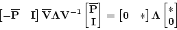
Then
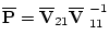 is a solution of the
CTARE. is a solution of the
CTARE.
|
Proof

|
 ensures that