|
You are here :
Control System Design - Index | Book Contents |
Appendix D
| Section D.3
D. Properties of Continuous-Time Riccati Equations
D.3 The stabilizing solution of the CTARE
We see from Section D.2 that we have as many
solutions to the CTARE as there are ways of partitioning the
eigevalues of H into the groups
 and
and
 .
Provided that .
Provided that  is stabilizable and that
 has no unobservable modes in the
imaginary axis, then
has no unobservable modes in the
imaginary axis, then
 has no eigenvalues in the imaginary
axis. In this case, there exists a unique way of partitioning the
eigenvalues so that
contains only the stable
eigenvalues of
.
We call the corresponding (unique) solution
of the CTARE the stabilizing solution and denote it by
has no eigenvalues in the imaginary
axis. In this case, there exists a unique way of partitioning the
eigenvalues so that
contains only the stable
eigenvalues of
.
We call the corresponding (unique) solution
of the CTARE the stabilizing solution and denote it by
 . .
Properties of the stabilizing solution
are given in the following.
Lemma D.4
| (a) |
The stabilizing solution has the property that the closed
loop
 matrix,
 |
 |
(D.3.1) |
|
|
where |
 |
(D.3.2) |
|
|
has eigenvalues in the open left-half plane. |
| (b) |
If
is detectable, then the
stabilizing solution is the only nonnegative solution of the
CTARE. |
| (c) |
If
has no unobservable modes
inside the stability boundary, then the stabilizing solution is
positive definite, and conversely. |
| (d) |
If
 has an unobservable mode
outside the stabilizing region, then in addition to the stabilizing
solution, there exists at least one other nonnegative solution of
the CTARE. However, the stabilizing solution,
has the property that
has an unobservable mode
outside the stabilizing region, then in addition to the stabilizing
solution, there exists at least one other nonnegative solution of
the CTARE. However, the stabilizing solution,
has the property that |
 |
(D.3.3) |
|
|
where
 is any other solution of the CTARE.
 |
|
|
|
|
Proof
For part (a), we argue as follows:
Consider (D.1.11) and (D.1.14). Then
 |
(D.3.4) |
which implies that
 |
(D.3.5) |
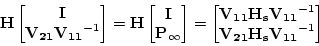
If we consider only the first row in (D.3.5), then, using
(D.1.8), we have
 |
(D.3.6) |
Hence, the closed-loop poles are the eigenvalues of
 and, by construction, these are stable. and, by construction, these are stable.
We leave the reader to pursue parts (b), (c), and (d) by studying
the references given at the end of Chapter 24.

|