|
You are here : Control System Design - Index | Book Contents | Appendix D | Section D.5 D. Properties of Continuous-Time Riccati Equations
|

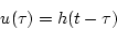
 by using a linear filter of the
following form:
by using a linear filter of the
following form:
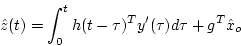
 is the impulse response of the filter and where
 is a given estimate of the initial state. Indeed, we
will assume that (22.10.17) holds, that is, that the initial
state
is a given estimate of the initial state. Indeed, we
will assume that (22.10.17) holds, that is, that the initial
state  satisfies
 ,
so that
,
so that
 is close to
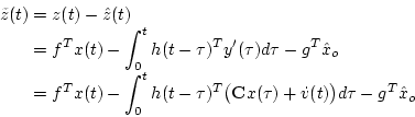
 and
and  in the
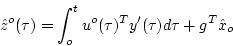
integral. Hence, we introduce another variable,
in the
integral. Hence, we introduce another variable,  ,
by
using the following equation
,
by
using the following equation

 is the reverse time form of
  :
:
 |
(D.5.7) |
Substituting (D.5.5) into (D.5.4) gives
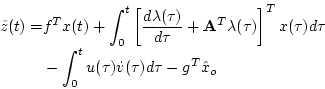
Using integration by parts, we then obtain
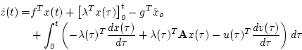
Finally, using (22.10.5) and (D.5.6), we obtain
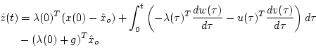
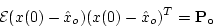
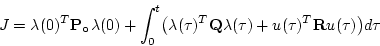
Hence, squaring and taking mathematical expectations, we obtain
(upon using (D.5.3),
(22.10.3) and (22.10.4) ) the following:
The last term in (D.5.11) is zero if
 .
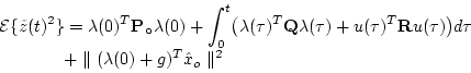
Thus,
we see that the design of the optimal linear filter can be
achieved by minimizing
.
Thus,
we see that the design of the optimal linear filter can be
achieved by minimizing
where
 satisfies the reverse-time equations
(D.5.5) and (D.5.6).
satisfies the reverse-time equations
(D.5.5) and (D.5.6).
We recognize the set of equations formed by (D.5.5), (D.5.6), and (D.5.12) as a standard linear regulator problem, provided that the connections shown in Table D.1 are made.


Table D.1: Duality in quadratic regulators and filters
Finally, by using the (dual) optimal control results presented earlier, we see that the optimal filter is given by
where
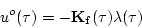
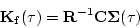
and
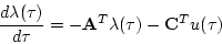
 satisfies the dual form of
(D.0.1), (22.4.18):
satisfies the dual form of
(D.0.1), (22.4.18):
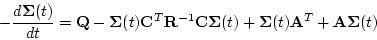

Substituting (D.5.14) into (D.5.5), (D.5.6) we see that
 |
(D.5.21) |
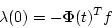
We see that  is the output of a linear homogeneous
equation. Let
is the output of a linear homogeneous
equation. Let
 ,
and define
,
and define
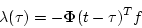
 as the
state transition matrix from
as the
state transition matrix from  for the time-varying system
having
for the time-varying system
having  equal to
![$\left[
\ensuremath{\mathbf{A-K}} _f(t-\nu)^T\ensuremath{\mathbf{C}}\right] $](appendixD-img150.png) .
Then
.
Then
 |
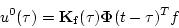 |
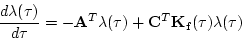
Hence, the optimal filter satisfies
 |
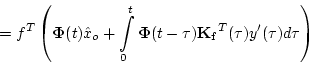 |
 |
where
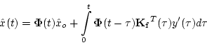
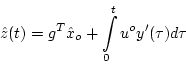
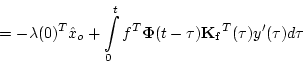
We then observe that (D.5.24) is actually the solution of
the following state space (optimal
filter).
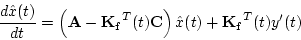


We see that the final solution depends on  only through
(D.5.27). Thus, as predicted, (D.5.25),
(D.5.26) can be used to generate an optimal estimate of any
linear combination of states.
only through
(D.5.27). Thus, as predicted, (D.5.25),
(D.5.26) can be used to generate an optimal estimate of any
linear combination of states.
Of course, the optimal filter (D.5.25) is identical to that given in (22.10.23)
All of the properties of the optimal filter follow by analogy from the (dual) optimal linear regulator. In particular, we observe that (D.5.16) and (D.5.17) are a CTDRE and its boundary condition, respectively. The only difference is that, in the optimal-filter case, this equation has to be solved forward in time. Also, (D.5.16) has an associated CTARE, given by

Thus, the existence, uniqueness, and properties of stabilizing solutions for (D.5.16) and (D.5.28) satisfy the same conditions as the corresponding Riccati equations for the optimal regulator.