2.5 Prototype Solution to the Control Problem via Inversion

You are here : Control System Design - Index | Book Contents | Chapter 2 | Section 2.5

2. Introduction to the Principles of Feedback

2.5 Prototype Solution to the Control Problem via Inversion

One particularly simple, yet insightful way of thinking about control problems is via inversion. To describe this idea we argue as follows:

say that we know what effect an action at the input of a system produces at the output, and
say that we have a desired behavior for the system output; then one simply needs to invert the relationship between input and output to determine what input action is necessary to achieve the desired output behavior.

In spite of the apparent naivety of this argument, its embellished ramifications play a profound role in control-system design. In particular, most of the real-world difficulties in control relate to the search for a strategy that captures the intent of the above inversion idea, while respecting a myriad of other considerations, such as insensitivity to model errors, disturbances, and measurement noise.

To be more specific, let us assume that the required behavior is specified by a scalar target signal or reference r(t), that has an additive disturbance d(t). Say we also have available a single manipulated variable, u(t). We denote by y(t) a function of time: $y=\{y(t):t\in\mathbb{R}\}$ .

In describing the prototype solution to the control problem below, we will make a rather general development that, in principle, can apply to general nonlinear dynamical systems. In particular, we will use a function, $f\langle \circ \rangle$ , to denote an operator mapping one function space to another. So as to allow this general interpretation, we introduce the following notation:

The symbol y (without brackets) will denote an element of a function space: $y\stackrel{\rm\triangle}{=}\left\{ y(t):\; \mathbb{R}\rightarrow\mathbb{R}\right\}$ . An operator, $f\langle \circ \rangle$ , will then represent a mapping from a function space, say $\chi$ , onto $\chi$ .

What we suggest is that the reader, on a first reading, simply interpret f as a static linear gain linking one real number, the input u to another real number, the output y. On a subsequent reading, the more general interpretation, using nonlinear dynamic operators, can be used.

Let us also assume (for the sake of argument) that the output is related to the input by a known functional relationship of the form

$\begin{displaymath}y=f\langle u\rangle +d \end{displaymath}$

(2.5.1)

where fis a transformation or mapping (possibly dynamic) that describes the input-output relations in the plant.¹ We call a relationship of the type given in (2.5.1) a model.

The control problem then requires us to find a way to generate y=r. In the spirit of inversion, a direct, although somewhat naive, approach to obtain a solution would thus be to set

$\begin{displaymath}y=r=f\langle u\rangle +d \end{displaymath}$

(2.5.2)

from which we could derive a control law, by solving for u. This leads to

$\begin{displaymath}u=f^{-1}\langle r-d\rangle \end{displaymath}$

(2.5.3)

This idea is illustrated in Figure 2.6.

**Figure 2.6:** Conceptual controller

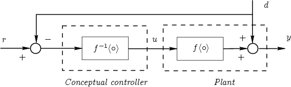
This is a conceptual solution to the problem. However, a little thought indicates that the answer given in (2.5.3) presupposes certain stringent requirements for its success. For example, inspection of equations (2.5.1) and (2.5.3) suggests the following requirements:

	R1	The transformation f clearly needs to describe the plant exactly.
	R2	The transformation f should be well-formulated in the sense that a bounded output is produced when u is bounded--we then say that the transformation is stable.
	R3	The inverse f^-1 should also be well-formulated in the sense used in R2.
	R4	The disturbance needs to be measurable, so that u is computable.
	R5	The resulting action u should be realizable and should not violate any constraint.

Of course, these are very demanding requirements. Thus, a significant part of Automatic Control theory deals with the issue of how to change the control architecture so that inversion is achieved but in a more robust fashion and so that the stringent requirements set out above can be relaxed.

To illustrate the meaning of these requirements in practice, we briefly review a number of situations.

Example 2.1 (Heat exchanger) Consider the problem of a heat exchanger in which water is to be heated by steam having a fixed temperature. The plant output is the water temperature at the exchanger output and the manipulated variable is the air pressure (3 to 15 [psig]) driving a pneumatic valve that regulates the amount of steam feeding the exchanger.

In the solution of the associated control problem, the following issues should be considered:

Pure time delays might be a significant factor, because this plant involves mass and energy transportation. However a little thought indicates that a pure time delay does not have a realizable inverse (otherwise we could predict the future), and hence R3 will not be met.
It can easily happen that, for a given reference input, the control law (2.5.3) leads to a manipulated variable outside the allowable input range (3 to 15 [psig] in this example). This will lead to saturation in the plant input. Condition R5 will then not be met.

$\Box \Box \Box$

Example 2.2 (Flotation in mineral processing) In copper processing, one crucial stage is the flotation process. In this process, the mineral pulp (water and ground mineral) is continuously fed to a set of agitated containers where chemicals are added to separate (by flotation) the particles with high copper concentration. From a control point of view, the goal is to determine the appropriate addition of chemicals and the level of agitation to achieve maximal separation.

Characteristics of this problem are as follows:

The process is complex (physically distributed, time varying, highly nonlinear, multivariable, and so on) and hence it is difficult to obtain an accurate model for it. Thus, R1 is hard to satisfy.

One of the most significant disturbances in this process is the size of the mineral particles in the pulp. This disturbance is actually the output of a previous stage (grinding). To apply a control law derived from (2.5.3), one would need to measure the size of all these particles or (at least) to obtain some average measure of this. Thus, condition R4 is hard to satisfy.

Pure time delays are also present in this process, and thus condition R3 cannot be satisfied.

$\Box \Box \Box$

One could imagine various other practical cases where one or more of the requirements listed above cannot be satisfied. Thus, the only sensible way to proceed is to accept that there will inevitably be intrinsic limitations and to pursue the solution within those limitations. With this in mind, we will impose constraints that will allow us to solve the problem subject to the limitations that the physical set-up imposes. The most commonly used constraints are as follows:

	L1	to restrict attention to those problems where the prescribed behavior (reference signals) belong to restricted classes and where the desired behavior is achieved only asymptotically;
	L2	To seek approximate inverses.

In summary, we can conclude the following:

In principle, all controllers implicitly generate an inverse of the process, in sofar as this is feasible. Controllers differ with respect to the mechanism used to generate the required approximate inverse.

¹ We introduce this term here loosely. A more rigorous treatment will be deferred to Chapter 19.

Previous - Section 2.4

Up - Chapter 2

Next - Section 2.6