|
You are here : Control System Design - Index | Book Contents | Chapter 2 | Section 2.6 2. Introduction to the Principles of Feedback
|
 |
(2.6.1) |
Thus,
 |
(2.6.2) |
from which we finally obtain
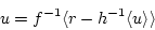
Equation (2.6.3)
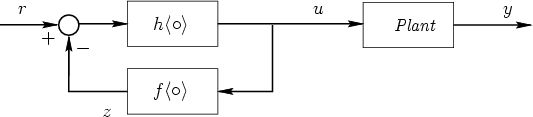
suggests that the loop in Figure 2.7
implements an approximate inverse of
 ,
that is,
,
that is,
 ,
if
,
if
 |
(2.6.4) |
We see that this is achieved if h-1 is small, that is, if h is a high-gain transformation.
Hence, if f characterizes our knowledge of the plant and if h is a high-gain transformation, then the architecture illustrated in Figure 2.7 effectively builds an approximate inverse for the plant model without requiring that the model of the plant, f be explicitly inverted. We illustrate this idea by an example.
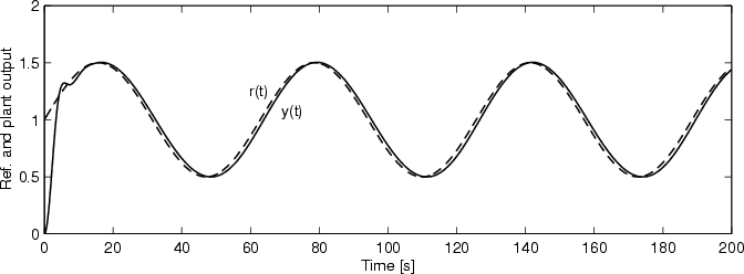
Example 2.3 Assume that a plant can be described by the model
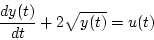
and that a control law is required to ensure that y(t) follows a slowly varying reference.
One way to solve this problem is to construct an inverse for the model
that is valid in the low-frequency region. Using the architecture
in Figure fig:inv1, we obtain an approximate inverse, provided that
 has large
gain in the low-frequency region. A simple solution is to choose
to be an integrator that has infinite gain at
zero frequency. The output of the controller is then fed to the
plant. The result is illustrated in Figure 2.8, which
shows the reference and the plant outputs. The reader might wish to
explore this example further by using the SIMULINK
file tank1.mdl on the accompanying CD.
has large
gain in the low-frequency region. A simple solution is to choose
to be an integrator that has infinite gain at
zero frequency. The output of the controller is then fed to the
plant. The result is illustrated in Figure 2.8, which
shows the reference and the plant outputs. The reader might wish to
explore this example further by using the SIMULINK
file tank1.mdl on the accompanying CD.