|
You are here : Control System Design - Index | Book Contents | Appendix C | Section C.8 C. Results from Analytic Function Theory
|
 .
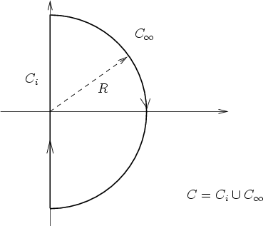
.  . This contour is shown in
  with
with  .
.
 ;
; 

 ,
i.e.,
,
i.e.,
 is like
  .
Then
.
Then
 is analytic inside
 |
(C.8.7) |
Because
 ,
the integral over
,
the integral over  can be
decomposed into the integral along the imaginary axis ,
can be
decomposed into the integral along the imaginary axis ,  ,
and
the integral along the semicircle of infinite radius,
,
and
the integral along the semicircle of infinite radius,  .
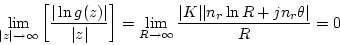
Because
.
Because  satisfies (C.8.3), this second integral
vanishes, because the factor
satisfies (C.8.3), this second integral
vanishes, because the factor
 is of order
  at
at  .
.
Then
The result follows upon replacing  and
and  by their real;
and imaginary-part decompositions.
by their real;
and imaginary-part decompositions.

Remark C.1
One of the functions that satisfies
(C.8.3) but does not satisfy (C.8.1)
is
 , where
  is a rational
function of relative degree
is a rational
function of relative degree  . We notice that, in this
case,
. We notice that, in this
case,
 |
(C.8.9) |
where  is a finite constant and
  is an angle in
![$[-\frac{\pi}{2}, \frac{\pi}{2}] $](appendixC-img192.png) .
.
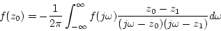
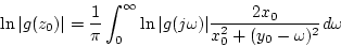
Remark C.2 Equation (C.8.4) equates two complex quantities. Thus, it also applies independently to their real and imaginary parts. In particular,
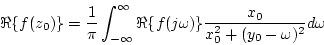
This observation is relevant to many interesting cases. For
instance, when is as in remark C.1,
 |
(C.8.11) |
For this particular case, and assuming that is a real function
of  , and that
  , we have that (C.8.10) becomes
 |
(C.8.12) |
where we have used the conjugate symmetry of .