|
You are here :
Control System Design - Index | Book Contents | Appendix B | Section B.3
B. Smith McMillan Forms
B.3 Smith Form for Polynomial Matrices
Using the above notation, we can manipulate polynomial matrices in
ways that mirror the ways we manipulate matrices of reals. For
example, the following result describes a diagonal form for
polynomial matrices.
Theorem B.1 (Smith form)
Let

be a

polynomial matrix
of rank  ;
then

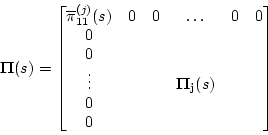
is equivalent to either a matrix

(for  )
or to a matrix

(for  ), with
 |
(B.3.1) |
 |
(B.3.2) |
where  and
and  are matrices with all their
elements equal to zero.
Furthermore
 are monic polynomials for
 ,
such that ,
such that
 is a factor in
 ,
i.e. ,
i.e.
 divides
 . .
If  ,
then ,
then
 is equivalent to the square
matrix
 . .
Proof (by construction)
| (i) |
|
By performing row and column interchange
operations on
 ,
bring to position (1,1) the least degree
polynomial entry in ,
bring to position (1,1) the least degree
polynomial entry in
 .
Say this minimum degree is .
Say this minimum degree is

|
| (ii) |
|
Using elementary operation (e03) (see
Definition B.3),
reduce the term in the position (2,1) to degree
 .
If the term in position (2,1) becomes zero, then go
to the next step, otherwise, interchange rows 1 and 2 and repeat the
procedure until the term in position (2,1) becomes zero. .
If the term in position (2,1) becomes zero, then go
to the next step, otherwise, interchange rows 1 and 2 and repeat the
procedure until the term in position (2,1) becomes zero.
|
| (iii) |
|
Repeat step (ii) with the other elements in the first
column.
|
| (iv) |
|
Apply the same procedure to all the elements but the
first one in the first row.
|
| (v) |
|
Go back to step (ii) if nonzero entries due to
step (iv) appear in the first column. Notice that the degree of the entry
(1,1) will fall in each cycle, until we finally end up with a matrix
which can be partitioned as
 |
(B.3.3) |
where
 is a monic polynomial.
|
| (vi) |
|
If there is an element of
 which is of
lesser degree than
 ,
then add the column
where
this element is to the first column and repeat steps (ii) to (v).
Do this until the form (B.3.3) is achieved with ,
then add the column
where
this element is to the first column and repeat steps (ii) to (v).
Do this until the form (B.3.3) is achieved with
 of less or, at most, equal degree to that
of every element in
 .
This will yield further
reduction in the degree of the entry in position (1,1). .
This will yield further
reduction in the degree of the entry in position (1,1).
|
| (vii) |
|
Make
 . .
|
| (viii) |
|
Repeat
the procedure from steps (i) through (viii) to matrix
 . .
|
Actually the polynomials
 in the above result
can be obtained in a direct fashion, as follows:
| (i) |
|
Compute all minor determinants of
 . .
|
| (ii) |
|
Define  as the (monic) greatest common divisor
(g.c.d.) of all
 minor determinants of
 .
Make .
Make
 . .
|
| (iii) |
|
Compute the polynomials
 as
as
 |
(B.3.4) |
|
|
 be a
be a
 polynomial matrix
of rank
  ;
then
 is equivalent to either a matrix
 (for
(for  )
or to a matrix
 (for
(for  ), with


 and
and  are matrices with all their
elements equal to zero.
 are monic polynomials for
 ,
such that
 ,
i.e.
 ,
then
 .
.

 .
If the term in position (2,1) becomes zero, then go
to the next step, otherwise, interchange rows 1 and 2 and repeat the
procedure until the term in position (2,1) becomes zero.

 is a monic polynomial.
 which is of
lesser degree than
 .
.
 as the (monic) greatest common divisor
(g.c.d.) of all
 minor determinants of
 .
.
