|
You are here : Control System Design - Index | Book Contents | Appendix B | Section B.4 B. Smith-McMillan FormsB.4 Smith-McMillan Form for Rational MatricesA straightforward application of Theorem B.1 leads to the following result, which gives a diagonal form for a rational transfer-function matrix:
Theorem 2.2 (Smith-McMillan form)
Let ![$\mathbf{G}(s)=[G_{ik}(s)]$](appendixb-img49.png) be an
be an  matrix transfer
function, where
matrix transfer
function, where  are rational scalar transfer
functions:
are rational scalar transfer
functions:
where
Then,
where
Furthermore,
ProofWe write the transfer-function matrix as in (B.4.1). We
then perform the algorithm outlined in Theorem B.1 to
convert
We use the symbol
We illustrate the formula of the Smith-McMillan form by a simple example.
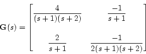
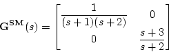
Example B.1 Consider the following transfer-function matrix
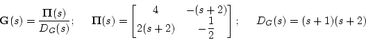
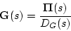
We can then express
The polynomial matrix
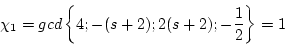
This leads to
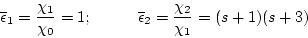
From here, the Smith-McMillan form can be computed to yield
|
 is an
is an  and
and  is the least common multiple of the
denominators of all elements
is the least common multiple of the
denominators of all elements  is equivalent to a matrix
 ,
with
,
with
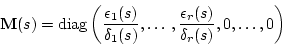
 is a pair of monic and
coprime polynomials for
is a pair of monic and
coprime polynomials for
 .
.
 is a factor of
 and
and
 is a factor of
 .
.

 to denote
 ,
which is the
Smith-McMillan form of the transfer-function matrix
,
which is the
Smith-McMillan form of the transfer-function matrix