|
You are here :
Control System Design - Index | Book Contents |
Appendix B
| Section B.6
B. Smith-McMillan Forms
B.6 Matrix Fraction Descriptions (MFD)
A model structure that is related to the Smith-McMillan form is
that of a matrix fraction description (MFD). There are
two types, namely a right matrix fraction description (RMFD) and a
left matrix fraction description (LMFD).
We recall that a matrix
 and its
Smith-McMillan form
and its
Smith-McMillan form
 are equivalent matrices. Thus,
there exist two unimodular matrices,
are equivalent matrices. Thus,
there exist two unimodular matrices,
 and
and
 ,
such
that ,
such
that
 |
(B.6.1) |
This implies that
if
is an  proper transfer-function
matrix, then there exist a
matrix
proper transfer-function
matrix, then there exist a
matrix
 and
an
matrix
and
an
matrix
 ,
such as ,
such as
 |
(B.6.2) |
where
and
are, for example,
given by
![\begin{displaymath}\ensuremath{\mathbf{\tilde{L}}(s)} =[\ensuremath{\mathbf{L}(s...
...ath{\mathbf{\tilde{R}}(s)} =[\ensuremath{\mathbf{R}(s)} ]^{-1}
\end{displaymath}](appendixb-img92.png) |
(B.6.3) |
We next define the following two matrices:
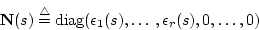 |
(B.6.4) |
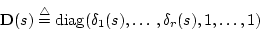 |
(B.6.5) |
where
 and
and
 are
matrices.
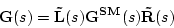
Hence,
can be written as
are
matrices.
Hence,
can be written as
![\begin{displaymath}
\ensuremath{\mathbf{G^{SM}}(s)} = \ensuremath{\mathbf{N}(s)} [\ensuremath{\mathbf{D}(s)} ]^{-1}
\end{displaymath}](appendixb-img97.png) |
(B.6.6) |
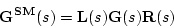
Combining (B.6.2) and (B.6.6), we can write
![\begin{displaymath}
\ensuremath{\mathbf{G}(s)} =\ensuremath{\mathbf{\tilde{L}}(...
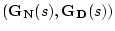
...suremath{\mathbf{G_N}(s)} [\ensuremath{\mathbf{G_D}(s)} ]^{-1}
\end{displaymath}](appendixb-img98.png) |
(B.6.7) |
where
![\begin{displaymath}
\ensuremath{\mathbf{G_N}(s)}\stackrel{\rm\triangle}{=}\ensu...
...uremath{\mathbf{\tilde{R}}(s)} ]^{-1}\ensuremath{\mathbf{D}(s)}\end{displaymath}](appendixb-img99.png) |
(B.6.8) |
Equations (B.6.7) and (B.6.8) define what is
known
as a right matrix fraction description (RMFD)
.
It can be shown that
 is always column-equivalent to a
column proper matrix
is always column-equivalent to a
column proper matrix
 .
(See definition B.7). This implies that the degree of the pole
polynomial .
(See definition B.7). This implies that the degree of the pole
polynomial  is equal to the sum of the degrees of the
columns of
.
is equal to the sum of the degrees of the
columns of
.
We also observe that the RMFD is not unique, because, for any nonsingular
matrix
 ,
we can write ,
we can write
 as
as
![\begin{displaymath}\ensuremath{\mathbf{G}(s)} = \ensuremath{\mathbf{G_N}(s)}\ens...
...suremath{\mathbf{\ensuremath{\boldsymbol{\Omega}}}(s)} ]^{-1}
\end{displaymath}](appendixb-img104.png) |
(B.6.9) |
where
is said to be a right common
factor. When the only right common factors of
 and
are unimodular matrices, then, from definition
definition B.7, we have that
and
are
right coprime. In this case, we say
that the RMFD
and
are unimodular matrices, then, from definition
definition B.7, we have that
and
are
right coprime. In this case, we say
that the RMFD
 is irreducible.
It is easy to see that when a RMFD is irreducible, then
Remark B.1 A left matrix fraction description (LMFD)
can be built similarly, with a different grouping of the matrices
in (B.6.7). Namely,
![\begin{displaymath}\ensuremath{\mathbf{G}(s)} =\ensuremath{\mathbf{\tilde{L}}(s)...
...verline{G}_D}(s)} ]^{-1}\ensuremath{\mathbf{\overline{G}_N}(s)}\end{displaymath}](appendixb-img110.png) |
(B.6.10) |
where
![\begin{displaymath}
\ensuremath{\mathbf{\overline{G}_N}(s)}\stackrel{\rm\triang...
...math{\mathbf{D}(s)} [\ensuremath{\mathbf{\tilde{L}}(s)} ]^{-1}
\end{displaymath}](appendixb-img111.png) |
(B.6.11) |

The left and right matrix descriptions have been initially derived
starting from the Smith-McMillan form. Hence, the factors are polynomial
matrices. However, it is immediate to see that they provide a more
general description. In particular,
,
,
 and
are generally matrices
with rational entries. One possible way to obtain this type of
representation is to divide the two polynomial matrices forming
the original MFD by the same (stable) polynomial.
and
are generally matrices
with rational entries. One possible way to obtain this type of
representation is to divide the two polynomial matrices forming
the original MFD by the same (stable) polynomial.
An example summarizing the above concepts is considered next.
Example 2.2 Consider a  MIMO system having the transfer function MIMO system having the transfer function
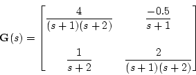 |
(B.6.12) |
| B.2.1 |
Find the Smith-McMillan form by performing elementary row and column operations.
|
| B.2.2 |
Find the poles and zeros.
|
| B.2.3 |
Build a RMFD for the model.
|
Solution
| B.2.1 |
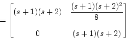
We first compute its Smith-McMillan form by performing elementary row and
column operations. Referring to equation (B.6.1), we
have that
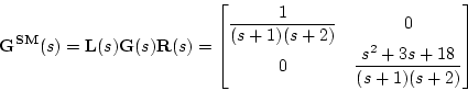 |
(B.6.13) |
with
![\begin{displaymath}\ensuremath{\mathbf{L}(s)} = \begin{bmatrix}\displaystyle{\fr...
...{8}} \\ [2mm] \displaystyle{0} & \displaystyle{1} \end{bmatrix}\end{displaymath}](appendixb-img116.png) |
(B.6.14) |
|
| B.2.2 |
We see that the observable and controllable part of the system has
zero and pole polynomials given by
 |
(B.6.15) |
which, in turn, implies that there are two transmission
zeros, located at
 ,
and four poles, located at ,
and four poles, located at
 and
and  . .
|
| B.2.3 |
We can now build a RMFD by using
(B.6.2).
We first notice
that
![\begin{displaymath}
\ensuremath{\mathbf{\tilde{L}}(s)} =[\ensuremath{\mathbf{L}...
...{8}} \\ [2mm] \displaystyle{0} & \displaystyle{0} \end{bmatrix}\end{displaymath}](appendixb-img121.png) |
(B.6.16) |
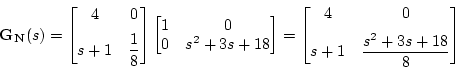
Then, using (2.24), with
![\begin{displaymath}
\ensuremath{\mathbf{N}(s)} =\begin{bmatrix}\displaystyle{1}...
...m] \displaystyle{0} &
\displaystyle{(s+1)(s+2)}
\end{bmatrix}\end{displaymath}](appendixb-img122.png) |
(B.6.17) |
the RMFD is obtained from (B.6.7),
(B.6.16), and
(B.6.17), leading to
 |
(B.6.18) |
and
![\begin{displaymath}\ensuremath{\mathbf{G_D}(s)} =\begin{bmatrix}\displaystyle{1}...
...m]\displaystyle{0} & \displaystyle{(s+1)(s+2)}
\end{bmatrix}
\end{displaymath}](appendixb-img124.png) |
(B.6.19) |
 |
(B.6.20) |
These can then be turned into proper transfer-function matrices by
introducing common stable denominators.
|
|
 is a zero of
 is a pole of
 .
.